

REPORT
Development of Feature Representations from
Emotionally coded Facial Signals and Speech
January 1999
Report for the TMR PHYSTA project
“Principled Hybrid systems: Theory and Applications”
Research contract FMRX-CT97-0098 (DG 12 – BDCN)
0 Preliminaries
*1. Introduction
*2. Classical Methods for Face and Speech Analysis
*2.1 Normalisation of static images
*2.2 Feature localisation and tracking
*2.3 Feature Extraction for Face Representation
*2.3.1 Methods for Edge Detection
*2.3.2 Multi-scale Pyramids and Wavelets
*2.3.3 Keypoints and Steerable Filters
*2.4 Feature extraction of speech signals
*2.4.1. Oscillogram (Waveform)
*2.4.2. Spectrum
*2.4.3. Spectrogram
*2.4.2 Fundamental Frequency (Pitch. F0)
*2.4 Motion Estimation
*2.5 Moving Object Feature Extraction
*2.6 Motion Feature Extraction in Facial Image Sequences
*2.6.1 Optic Flow Feature Extraction of Facial Expressions
*2.7 Face processing utilising profile views
*2.7.1 Extraction of Benchmark Points
*2.7.2 Texture Map Generation
*2.7.3 Modification and Rendering of the Head Mesh
*3. Supervised and unsupervised architectures for face perception
*3.1 Principle Component Analysis
*3.2 Backpropagation Feature Extraction
*3.3 Local Feature Analysis
*3.4 Independent Component Analysis
*4. Multiresolution based hierarchical Neural Networks for Vision
*4.1 Multiresolution Analysis
*4.2 Hierarchical Multiresolution Neural Classifiers
*5. Features in Speech Perception
*5.1. Emotion: In what Context?
*5.2. Deafened People’s Speech
*5.3. ASSESS Applied to Emotion
*5.4. Prosody in ‘Flattened Affect’
*5.5. Summary
*6. The ASSESS System
*7. Conclusion
*References
*Appendix: ……………………………………………………………………………41
This report is part of the PHYSTA project, which aims to develop an artificial emotion decoding system The system will use two types of input, visual (specifically facial expression) and acoustic (specifically non-verbal aspects of the speech signal).
PHYSTA will use hybrid technology, i.e. a combination of classical (AI) computing and neural nets (NN). Broadly speaking, the classical component allows for the use of known procedures and logical operations which are suited to language processing. The neural net component allows for learning at various levels, for instance the weights that should be attached to various inputs, adjacencies, and probabilities of particular events given certain information.
The report presents results of the extraction and use of visual and acoustic features. It is a fusion of results under the readings “NN-based extraction and evaluation of features from signals” and “Higher-order representation derived by hierarchical neural Networks”, which are under task 2 (WP2) of the original PHYSTA project programme. It uses material contained in the previous reports “Review of AI and NN techniques for mapping features to symbols” and “Review of existing techniques for human emotion understanding and applications in human-computer interaction”.
A review of classical methods for face analysis will be presented next, incorporating normalisation and feature extraction methods like edge detection, motion estimation and advanced techniques. Section three explores the use of supervised and unsupervised techniques for static face perception and facial emotion extraction. The architectures covered are principle component analysis, backpropagation of error learning, local feature analysis, and independent component analysis. In section four the application of multiresolution based hierarchical neural networks to vision tasks are explored. Finally section five gives an overview of speech related emotion understanding using the ASSESS system which is described in chapter 6 followed by a general conclusion.
The recognition of facial expressions has been subject to scientific study since the pioneering work of Charles Darwin in the 19th century. Topics of current research are the localisation of brain regions involved in the processing of facial expressions , the automated extraction of expressions from images, and psycho-logical studies of expression content from auditory and visual data .
Despite the relatively small variability of face images showing neutral facial expressions, most humans have no problems recognising faces viewed under varying illumination, size, and viewing angle or even showing different facial expressions. A simple pattern matching strategy for face recognition utilising only the raw image intensities will not be able to generalise well to new views of a known face, therefore a closer look at the neurobiology of face processing may reveal insights into the design principles for general systems for face perception.
Recent neurophysiological studies on the representation of objects in the inferior temporal cortex of the primate brain revealed highly specific neurones, responsive to critical features which are complex combinations of simple features like orientation, texture, size, and colour. These complex visual features are organised into columns, and take the form of sparse population codes for the representation of individual faces.
Aspects of expression recognition from face images are related to the recognition of faces, and we will give an overview of some methods for automated face recognition in the next sections. General problems with mugshot facial images are the appropriate normalisation of the images with respect to a reference view. This normalisation is necessary if the recognition method does not have its own normalisation mechanism and relies on the extracted features in the training phase.
Since facial expressions are dynamic, it is convenient to incorporate the temporal development of each expression in the analysis to improve performance. To normalise the images from a video stream, feature location and tracking mechanisms can be used to pre-process an image by transforming it to a suitable view. Mechanisms for face localisation and normalisation are further reviewed in section 2.2.
A second source for emotion recognition is speech, which can be analysed according to various strategies. One is to analyse speech of normal people under a variety of emotional conditions, say happy, neutral, angry, etc. Another is to compare the emotional content and response to speech of neutrals and of deaf people. A third is to compare emotional speech between normal controls and those with mental deficits, such as schizophrenia, autism and Alzheimer’s disease. Finally we have to face the problem of discerning the crucial clues in speech indicating specific emotionality. This is a broad area, involving time series analysis of the relevant speech signals.
We use the in-house ASSESS system here, although other signal processing systems such as TESPAR would be of interest to apply here. The TESPAR parameterisation goes beyond that of ASSESS in that it picks out the positions of all complex zeros of the signal; it does not use specific Fourier techniques, however.
2. Classical Methods for Face and Speech Analysis
The computerised analysis of faces and speech signals builds upon classical methods of image and sound analysis. Therefore we will give an overview of typical techniques which have been applied to extract features from images and auditory signals. First we examine classical methods for image normalisation and tracking. Next methods for feature extraction from static images like edge detection and wavelet analysis will be presented. Section 2.4. presents common representations of speech signals like oscillogram, spectrogram, and fundamental frequency or pitch analysis. The following sections will give examples of motion feature extraction from image sequences like optical flow methods and block-based motion analysis. The last section gives an example of an advanced classical method for face recognition using frontal and profile views incorporating the use of texture information of the face.
2.1 Normalisation of static images
A prerequisite for reliable automated face processing is the normalisation of the face to a predefined position and viewpoint. The procedure to achieve face normalisation can be decomposed into five successive processing steps, which are depicted in figure 1.
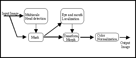
The first step is to extract the head from an image, which in principle could contain multiple faces having general viewing orientations and different sizes, by a multiscale head search. After cropping and warping the face to a standard size, the second step can be applied, which involves a search for salient facial features like the eyes, eyebrows, nose, chin, and the mouth. The extracted features can then be used to normalise the face to a standard viewing position by a similarity transformation (translation, rotation and scaling) or an affine transformation (similarity and shear). A more advanced technique is to use a generalised morphing procedure based on radial basis functions, which also can account for localised spatial deformations due to the modifications of facial expressions . The next steps depicted in figure 1 are masking the face and normalising its contrast, and the subsequent coding and recognition using a low-dimensional representation described in the previous sections. This representation can be used to reconstruct the original face image by inverse warping and contrast restoration.
2.2 Feature localisation and tracking
The first steps to normalise face images are to locate the head and salient facial features in the images. In general seven approaches can be distinguished:
The first approach that uses coloured facial markers on keypoints of the face is simple to implement and yields good results, but suffers from being limited to artificially controlled environments. However, this approach can be used to guide a more sophisticated technique. The use of skin hue to extract the position of the head has been shown to be largely constant across races. Therefore this approach has been widely used to extract an initial estimate of the head position. However, additional shape-based constraints may be used to reject hands or skin-coloured objects in the image. An obvious technique to locate the head is simple frame differencing of successive images, since for a static camera, the person is usually the only moving object in the scene. Again, shape-based and continuity constraints can be used to extract the head of the moving persons contour.
The template-based approach uses a database of simple two-dimensional geometrical models of the head or some salient parts of it (eyes, nose, etc.), and tries to match these models to the image. The templates can be defined on the raw image intensities or on the image gradients by edge filtering them. Since the faces can have different sizes, forms, and viewpoints, a large database of face templates is necessary to ensure sufficient detection performance. To over-come this limitation, two approaches using deformable templates have been proposed: the parameterised template approach proposed by Yuille uses a priori knowledge about the expected shape of a feature to guide the detection process, and the parameters of the model are fitted to the image by a dynamic energy minimisation procedure. This approach is largely insensitive to variations in scale, tilt and rotation of the head, and to lighting conditions. A related approach uses a dynamic spline-based contour model (snake) to track deformations of the face for further analysis. The model can be used for expression synthetisation from image sequences, but suffers from needing an explicit initialisation on a facial contour. The generalised symmetry operator assigns a symmetry magnitude and orientation at every pixel in an edge filtered image. Since strong symmetry edges are points of natural interest (eyes, mouth, nose), these points can be used to direct a higher level segmentation process.
2.3 Feature Extraction for Face Representation
The level of early visual processing includes the extraction of parameterised intrinsic images, which reflect specific local properties in the scene. Typical intrinsic parameters are surface discontinuities (edges and lines), measured distance (range), surface orientation (Shape), velocity (motion), and resolution (scale). The calculation of the intrinsic maps is usually performed in parallel using a spatially localised discretisation, which corresponds to the pixels in the image. Two methods can be distinguished: one-step methods like edge detection and iterative methods like relaxation procedures where the measured intrinsic parameters converge to a local consistent value.
A further class of low-level pre-processing is filtering, which appropriately transforms the image intensities to enhance specific features and to eliminate unwanted noise. Typical methods are thresholding or quantisation of the intensity levels and image smoothing. Contrasting the local methods of intrinsic maps, these techniques employ global image information like grayvalue statistics to enhance selected intensity ranges in the image.
The next step of intermediate visual analysis incorporates the determination of generic scene attributes and the grouping of the extracted visual features in the intrinsic maps to meaningful units. This uninterpreted segmentation and partitioning of the image represents the interface between low-level processing and high-level scene interpretation. The reliable automated extraction of unknown objects in a complex three dimensional scene is still an unsolved problem, since the homogenity of measured features like colour and intensity distribution, distance and orientation can vary due to inhomogeneous illumination, shading and mutual overlaps. However, if additional knowledge about the expected objects in the scene is available the segmentation can be simplified by imposing top-down constraints.
2.3.1 Methods for Edge Detection
The extraction of object boundaries in the intensity image is an elementary operation in computer vision. Also psychophysical studies show the importance of edges for visual perception. Objects and faces can often be identified in a raw sketch including only the major contour lines. Since the global extraction of contours in not possible due to the large number of possible contours, local edge detection is commonly used as a starting point for a subsequent edge grouping process which combines local edges into global contours. The proposed edge detectors can be classified into three groups:
The Roberts, Prewitt and the Sobel operator belong to the class of gradient operators, which measure grayvalue differences along orthogonal directions using two or four filter-masks. A disadvantage of these operators is their sensitivity to image noise and the weak orientation selectivity caused by the orthogonal basis and the small spatial averaging. The Kirsch operator employs four templates whose maximum response determines the orientation and the strength of the detected edge. A disadvantage of template-based filters is the discretisation of the orientations, which leads to false classification of intermediate orientations. The edge model proposed by Hueckel reduces the edge detection to an optimisation problem which can be solved using continuous spatial co-ordinates. Using a set of orthonormal, low frequency, basis functions inside a circular operator window, the mean quadratic deviation between image and a parameterised edge model is minimised. The resulting parameterisation is more accurate than the two-valued parameters of the gradient operator (direction and strength), but the computational expense is high since the optimisation has to be calculated at each discrete image position.
A general problem for most edge detectors is smooth intensity gradients caused by shades and illumination. To avoid the classification of these gradients as edges, a threshold has to be introduced which is difficult to estimate in advance. Furthermore, the grayvalue discontinuities can be distributed across multiple scales, enforcing a multiscale processing. The linear rotation invariant Laplace operator has been introduced by Marr and Hildreth to detect zero crossings of the second derivative of the intensity image. The zero crossings correspond to gradient maximum of the first derivative, which are the points of maximal change of image intensity. By successively smoothing the image by a Gaussian filter, a multiscale image pyramid can be generated which corresponds to the different spatial frequency channels of the human visual system. It has been shown that only filtering by a Gaussian filter exhibits well-behaved scale space properties and does not introduce new zero crossings along the scale space. Advantages of rotation invariant operators are their good localisation properties and their generation of closed contours. The disadvantages are the absence of any directional information and their strong sensitivity to noise.
The Canny operator combines many of the proposed methods for edge detection in a complex procedure using gradient operators of different widths, lengths, and orientation, and an adaptive threshold with hysteresis which is set according to the approximated image noise. The output of the different operators is combined according to a synthesis procedure, which uses the smaller operators to predict the output of the larger operators. The optimality of the Canny operator has been shown for the detection of intensity jumps. However, the detection of lines, gradients, diffuse edges, and combinations of these edge types leads to systematic errors in the localisation of the true edge. The quadratic filter, which uses odd and even functions as detectors for both orthogonal edge types (lines and jumps) and combines them by non-linear summation, is able to detect all kinds of edges in the image. A special case of this filter is the model of phase dependent local energy, which employs two orthogonal basis functions constituting a Hilbert pair. Psychophysical experiments further demonstrated that the human visual system detects features at points where the Fourier components have identical phase, corresponding to the maximal energy and not at points of maximal luminance. Since the kind of detected edge is characterised by the local phase, the original signal can be reconstructed and the analytical signal of value and phase can be used for image coding.
2.3.2 Multi-scale Pyramids and Wavelets
Since images are composed of objects and features at multiple scales, an analysis of visual information should be applied at these scales using different spatial frequencies. The human visual system also shows a separation into four different frequency channels with a logarithmic scaling of the spectrum into octave steps. To analyse the scale space two principal approaches can be distinguished:
The image pyramids, which have been introduced in the seventies by Rosenfeld employ a recursive strategy to build up a multiscale representation using successive filtering and smoothing of the image into a hierarchical structure. An advantage of this efficient representation is the direct readout of the different frequency channels and the logarithmic speedup along the scale space. Complementing the discrete multiscale pyramids is the continuous scale space, which are generated by continuous convolution of the image with a Gaussian filter of variable variance. The scale space filtering method also can be interpreted as the continuous solution of the diffusion- or heat equation using the original image as the starting point. The use of multiscale representation will be further discussed in section 4.
2.3.3 Keypoints and Steerable Filters
The description of the image content using locally defined parameters like position, orientation, curvature, size or scale, phase, and velocity has been proven to be a suitable representation for many image processing applications like edge detection, texture analysis, motion analysis, and image compression. A general problem during the development and implementation regards to the appropriate discretisation to optimise storage consumption and processing speed. An efficient strategy to synthesise any oriented filter using a linear combination of a set of steerable basis filters has been proposed by Freeman and Adelson which also allows to determine the minimal basis. This method has been recently expanded to allow the construction of any discrete multiscale representation using a fixed number of basis filters.
2.4 Feature extraction of speech signals
Phonetics is part of the linguistic sciences. It is concerned with the sounds produced by the human vocal organs, and more specifically, the sounds which are used in human speech . To visualise the speech signal it can be displayed as an oscillogram, a series of spectrums or as an spectrogram. A representation which is useful for further analysis, specially of the signals emotional content is the extraction of the fundamental frequency. These four representations are presented next, using a phonology system to generate the corresponding graphs.
The most common visual representation of a speech signal is the oscillogram or waveform. It shows the amplitude of the sound signal over the full temporal duration. Figure 2 shows the oscillogram of an example sentence of length 3.7 seconds.
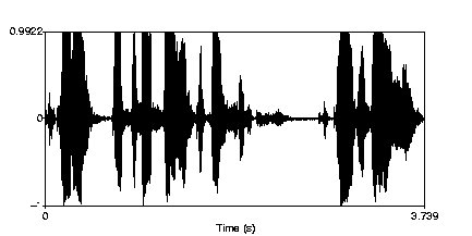
Figure 2 Oscillogram of the sentence „Activating virus defense system, prepare to download“.
According to general theories each periodical waveform may be described as the sum of a number of simple sine waves, each with a particular amplitude, frequency and phase. The spectrum gives a picture of the distribution of frequency and amplitude at a moment in time.
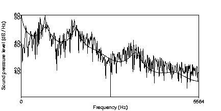
Figure 3 The spectrum of a short sequence of speech (5ms) overlayed with the LPC filtered contour.
In the spectrogram the time axis is the horizontal axis, and frequency is the vertical axis. The third dimension, amplitude, is represented by shades of darkness.
In the unvoiced fricative sounds, the energy is concentrated high up in the frequency band, and quite disorganized (noise-like) in its appearance. In other unvoiced sounds, e.g. the plosives, much of the speech sound actually consists of silence until strong energy appears at many frequency bands, as an "explosion". The voiced sounds appear more organized. The spectrum highs (dark spots) actually form horizontal bands across the spectrogram. These bands represent frequencies where the shape of the mouth gives resonance to sounds. The bands are called formants, and are numbered from the bottom up as F1, F2, F3 etc. The positions of the formants are different for different sounds and they can often be predicted for each phoneme.
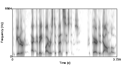
Figure 4 LPC smoothed Spectrogram of the sentece depicted in figure 2.
2.4.2 Fundamental Frequency (Pitch. F0)
Another representation of the speech signal is the one produced by a pitch analysis. Speech is normally looked upon as a physical process consisting of two parts: a product of a sound source (the vocal chords) and filtering (by the tongue, lips, teeth etc). The pitch analysis tries to capture the fundamental frequency of the sound source by analyzing the final speech utterance. The fundamental frequency is the dominating frequency of the sound produced by the vocal chords. It can be obtained from the harmonic series associated with voiced speech, by using a narrow band spectrogram. This analysis is quite difficult to perform. There are several problems in trying to decide which parts of the speech signal are voiced and which are not. It is also difficult to decipher the speech signal and try to find which oscillations originate from the sound source, and which are introduced by the filtering in the mouth. Several algorithms have been developed, but no algorithm has been found which is efficient and correct for all situations. The fundamental frequency is the strongest correlate to how the listener perceives the speakers' intonation and stress.
In the picture the fundamental frequency (often called F0 to be coherent with the terms for the formants, F1, F2 etc) is plotted against time. The F0 curve is visible only at points where the speech is voiced, i.e. where the vocal chords vibrate. The values for F0 lie between 100 and 150 Hz. This is common for a male speaker. The typical F0 range for a male is 80-200 Hz, and for females 150-350 Hz. Naturally, there is great variation in these figures.
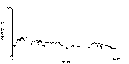
Figure 5 Fundamental Frequency of the sentence of figure 2.
Motion estimation is one of the most crucial parts of video coding and analysis algorithms. It greatly assists in redundant information reduction and in achieving high compression ratios, by predicting the values of pixels in each frame from corresponding values of a former ‘reference’ frame of the image sequence. It basically provides estimation of motion vectors; the latter represent the relative movement of a pixel or of a block of pixels between the two image frames.
To estimate the motion field, i.e., all motion vectors in a frame, a variety of techniques have been developed, based on computation of image intensity temporal and spatial differences. Such techniques include:
In block-based motion estimation, which is the most widely used method, blocks of 8x8 or 16x16 pixels are considered, and a search is performed to match each block of the new frame with one of the blocks belonging in a larger (say, 16x16 or 32x32 pixels) area of the reference (previous) frame; various criteria, such as sums of squared differences or sums of absolute differences, as well as various search methodologies, such as exhaustive, logarithmic, conjugate-direction, or one-dimensional hierarchical search, can be applied for block matching and motion field estimation.
2.5 Moving Object Feature Extraction
Motion analysis is the basic tool for the extraction of a moving object from video frames. It is generally anticipated that when the motion vectors are small (or zero), the respective regions do not contain significant information. As a consequence, these regions can be characterised as non-regions-of-interest (non-ROI). However, not all the blocks with large values of motion vectors can be characterised as regions of interest (ROI), since their values do not always correspond to real moving objects on which the human eye is concentrated, when viewing a specific scene.
The next Figure shows the motion vectors of Frame 2 of a well-known videophone sequence, Claire, where motion vectors have been calculated for 8x8 blocks within 16x16 area. It is observed that the values of the motion vectors in the background are sometimes large, although there is no motion in this area, or this motion is not perceivable by humans. This phenomenon occurs either due to changes of the image luminosity or due to the presence of noise. Hence, a simple algorithm that depends on the value of each motion vector in order to find ROI will fail. Neural networks are a possible solution for selecting those areas that contain moving objects as ROI and classifying the other areas as non-ROI.
In general blocks which belong to moving objects have two significant properties:
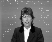
Figure 6 Motion vectors of frame 2 of Claire
According to the above, two 2-D parameters can be examined to select ROI areas in an image. These are the mean and the variance of the area which has the current block at its centre and includes four or eight adjacent (4 or 8 connectivity) blocks. These parameters should be computed and compared to a threshold T, which, however, is not constant for all kind of images. This disadvantage can be removed if a neural network is appropriately trained to classify correctly the blocks of images into ROI or non-ROI, based on the above features.
As an example, a neural network has been trained using groups of 3x3 blocks, each consisting of 8x8 pixels, at its input; a small number of frames of the Claire sequence have been used for training it. We next present the output of a learning vector quantizer (LVQ) network, when applied to frames not belonging in its training set. The output of the network is presented (in black) together with the motion vectors (white lines on the black blocks). Since the orientation and values of motion vectors in the background are not always random, it is necessary to train the neural network with a strict criterion to avoid misclassifying such areas belonging to background. A problem will then be faced from the boundaries of moving objects. This is so because a motion vector that belongs to the boundary of a moving object does not have the majority of adjacent motion vectors following the same orientation and magnitude. To solve this problem it is possible to extend the mask (output of the network) in these blocks that are adjacent to the previous one and have motion vectors with significant values. The results of this process are shown in the following Figure, where the extended blocks are illustrated in grey colour.
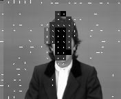
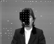
Figure 3 Moving areas extracted in frames 3 and 16 of Claire
2.6 Motion Feature Extraction in Facial Image Sequences
When specifically dealing with facial image sequences , non-rigid motion can be estimated using the following block-based motion analysis procedure:
![]() (1)
(1)
The motion vector of block ![]() is computed using logarithmic search (to decrease execution time) in a neighborhood of block
is computed using logarithmic search (to decrease execution time) in a neighborhood of block ![]()
‘Noisy’ motion vectors (i.e., poor estimates of motion vectors) inevitably arise due to the simplicity of motion estimation; to account for this, motion filtering should be adopted. Median filtering is a tool that can be applied first to the estimated motion vectors’ phase, so as to produce some kind of directional filtering, and then to their norm. Let ![]() denote the facial area, already segmented and aligned. It is straightforward to divide
denote the facial area, already segmented and aligned. It is straightforward to divide ![]() into predefined areas corresponding to facial parts, e.g., in six sub-areas corresponding to forehead, left/right eye/cheek, and mouth. A feature vector describing the motion between two consecutive frames can be formulated from the set of subareas in
into predefined areas corresponding to facial parts, e.g., in six sub-areas corresponding to forehead, left/right eye/cheek, and mouth. A feature vector describing the motion between two consecutive frames can be formulated from the set of subareas in ![]() . The above formulation will lead to a feature vector consisting of the averaged power within each sub area and for all directions. Facial parts with the most degrees of freedom (such as the mouth) can be assigned more features than the rest of the subareas. In this way facial anatomy is taken into consideration.
. The above formulation will lead to a feature vector consisting of the averaged power within each sub area and for all directions. Facial parts with the most degrees of freedom (such as the mouth) can be assigned more features than the rest of the subareas. In this way facial anatomy is taken into consideration.
2.6.1 Optic Flow Feature Extraction of Facial Expressions
The dynamic extraction of facial expression from image sequences naturally can be accomplished using optical flow estimation techniques. However, to interpret the extracted flow fields as facial expressions, the face has to be appropriately normalised by centring the image sequence on salient facial landmarks (see sections 2.1 and 2.7). A further problem is movement of the head relative to the static camera, which adds a directed component to the flow field, thereby covering the flow vectors of the facial expressions.
Figure 4 depicts the optic flow extracted from two image sequences, which show a person developing a smiling and a surprised face.
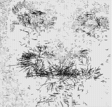
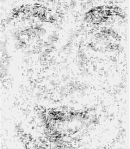
Figure 4 Opic flow vectors of facial expressions. Left: smile, Right surprise.
2.7 Face processing utilising profile views
Computer recognition of human faces has been an active research area for more than two decades. Humans can easily detect and identify faces in a scene with very little or no effort. However, designing an automated system to perform this task is very difficult. Several techniques have been proposed in order to improve the efficiency of these kinds of systems, most of which are based on single, frontal view facial images, with constraints posed on the lighting conditions as well as on the scale, rotation and orientation of the face in the image. Approaches to face recognition from frontal view images involve structural or statistical features of the human face as well as template matching and global transformations .
Alternative techniques for face processing utilise profile views for the recognition task. Most of these approaches depend exclusively on prominent visible features of the profile view such as nose and chin. However, recognition based only on these features ignores texture information and is therefore insufficient.
Frontal and profile images can be combined to create a texture map, which is cylindrically projected onto an appropriately adjusted 3D-head mesh. Initially, several protuberant points (let us call them benchmark points) are automatically detected in both views. These points are then used in two different ways; on the one hand to produce geometric measures (see Table 1, Figure 5), based on which prominent facial features on the head model are modified, and on the other hand to find the correct mapping between the pixels of the available views and the vertices of the head mesh.
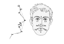
Figure 5 Benchmark points in profile and frontal views
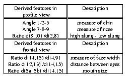
Table1: The extracted features; d(i,j) is the Euclidean distance between points i and j.
2.7.1 Extraction of Benchmark Points
The benchmark points in frontal and profile views are shown in Figure 5. Automated extraction of these points is a complex, but also important task, which crucially affects the accurate creation of a corresponding 3D model. Thus, the reliability of the point extraction procedure is a critical issue. In frontal views, where extraction is more elaborate, a dual approach can be considered to bestow the certainty needed; a hybrid method using template matching and Gabor filtering is fortified by the use of the eigenfeature theory.
As far as frontal images are concerned, the fundamental concept, upon which the automated localisation of the predetermined points is based, consists of two steps: the hierarchical and reliable selection of specific blocks of the image and the subsequent use of a standardised procedure for the extraction of the required benchmark points. Detection of blocks describing facial features relies on the effective extraction of some characteristic features. By adopting this reasoning, the choice of the most significant features has to be made. The importance of each of the commonly used facial features for recognition purposes has already been studied. The outcome of surveys proved the eyes to be the most crucial and easyly located facial feature. The techniques that we have developed and used for extraction of the features utilise a combination of template matching and Gabor filtering, as well as eigenfeature theory.
After having isolated the regions of interest from the frontal image, the localisation of the predetermined points ensues. The approximate centre of the eye’s pupil is searched for as the darkest point within the eye’s block, scanned both horizontally and vertically. The exact position of the nostrils is sought from the sides to the centre of the nose block. The mouth tips are determined in a similar manner. It is obvious that the whole search procedure is attempted to be as close to human perception as possible.
Feature points extracted from profile views were mainly used in early face recognition approaches. Different techniques were proposed to accomplish the extraction task. A frequently used approach considers benchmark points that lie exclusively in the profile outline. Thus the first step is to convert the profile view onto a binary image from which the profile line can be easily extracted. The conversion is applied by first enhancing the contrast between profile and background and then thresholding the gray scale image. The profile line in the binary image can be considered as a one-dimensional signal and the benchmark points on it as representing its local extremes. Localisation of the extreme points can be performed using non-linear approaches, such as morphological gradient, or linear ones, such as the Laplacian operator. An alternative technique involves measures of curvature of each point on the profile line.
The next step involves combining the two views into a single texture map. Further processing is required because cylindrical projection of an image introduces an amount of distortion. To compensate for it, a warping transformation is executed. The texture map is created by placing regions of the frontal and profile views side by side.
Columns from the frontal view are arranged in the centre region of the texture map while the ones of the profile are placed in the left and the right side of the texture map. At the centre column of the texture map we place the column of the frontal view which corresponds to the ‘nose point’ (benchmark point 8). The remaining columns are distorted accordingly. The last columns copied from the frontal view are the ones which correspond to the outer corners of the eyes.
In a similar way we arrange the columns of the profile in the left and right side of the texture map. Columns of the texture map, which have no assigned values are created using interpolation. Interpolation balances the illumination differences between frontal and profile view. Finally columns of the texture map which correspond to the back of the head are created by distorting the left most column of the profile to the left.
2.7.3 Modification and Rendering of the Head Mesh
The next task is to map the texture, the benchmark points and the extracted features to the generic head mesh; this is performed in three different steps. In the first step we apply (cylindrical) mapping co-ordinates to each vertex of the mesh. Mapping co-ordinates are essentially parameters in (u, v) space, also called texture space, that map every (x, y, z) point of the head mesh to a relevant (u, v) point in the texture map, i.e., the extended image. Cylindrical mapping does not cover areas of the head that are perpendicular to its axis, e.g., the top of the head, but for our purposes that is not an important issue.
Correct positioning of the texture map and, as a result, correct mapping of the texture elements to the vertices of the model is achieved through matching the benchmark points of the texture to those of a template that is created by unfolding the polygon mesh onto the imaginary mapping cylinder. The derived features are then used in a feedback manner to scale the relevant parts of the head mesh in order to match those of the specific human head that the system deals with. This creates the required mesh that is stable after a relatively small number of changes. Rendering the mesh is a straightforward procedure that can be achieved using either a commercial or a proprietary program. For the purposes of this project, we created a small modelling and rendering package, based on the HOOPS library. Positioning the mesh in an arbitrary angle (e.g. 15 degrees) can then easily be accomplished. Figure 6 shows the image of head mesh after the application of mapping co-ordinates. Figure 7 shows the generated synthetic view of a member of a facial database, created at the University of Bern by Mr. Bernard Achermann, (rotated by an angle of 15 degrees), following the above procedure.
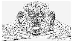
Figure 6 The generated Head Mesh
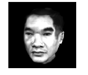
Figure 7 The Generated Synthetic View
During the last years, numerous architectures and algorithms for face recognition and expression recognition from facial images have been proposed. Surveys of this field can be found in. A general distinction into feature- and template-based approaches has been described by Brunelli and Poggio, but psychological experiments indicate that the human visual system processes faces at least to some extend holistically, favouring template-based approaches over feature-based techniques for their biological validity. We will therefore focus on advanced template-based techniques which can be further subdivided into global (PCA, Backpropagation) and local (LFA, ICA) template-based techniques.
3.1 Principle Component Analysis
The use of Principle Component Analysis (PCA) for face recognition has been described by serveral research groups in the last decade. The general idea behind this approach is to extract the main information in the training set as represented by some template images that capture most of the variability in the data. This is achieved by projecting the input images onto orthogonal basis images, which have the property of allowing the best possible reconstruction of the training images. The general approach of PCA is to calculate the eigenvectors of the covariance matrix of the input data, and to use only the K eigenvectors with the largest eigenvalues above some threshold to represent the input data and their principal directions. Since the calculation of the eigenvalues of a covariance matrix with large dimensional vectors is computationally intensive, this method can not in general be applied to image processing applications, where the size of the vectors equals the number of pixels of the training images.
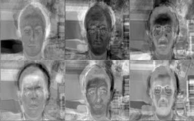
To allow the fast computation of the principal components of face images, a different approach has been proposed: the principle components are not calculated from the raw image intensity, but from the covariance matrix of the input images themselves. Since this quadratic matrix is only of size N x N, where N is the number of training images, the fast computation of the eigenvectors of the K largest eigenvalues is possible. The eigenvectors represent the K combinations of the N input images which capture most of the variability in these images, and allow the reconstruction of all training images with the least mean squared error. The PCA method, which has been termed the Eigenface method due to the similarity of the appearance of the K template images to „Ghost“-Faces, relies on the assumption that a low-dimensional representation of the face images using a small value of K, much smaller than N, suffices to capture most variation in the training images. This is not true in general, since the training images could be very dissimilar, resulting in a poor representation if only the eigenfaces with the K largest eigenvalues are considered. Therefore, it is necessary to align the images to a general viewpoint prior to the Eigenface decomposition by translating, scaling, and rotating the faces to a reference position. It has been demonstrated that although choosing the K largest eigenvalues is optimal for identifying physical categories of faces like sex, it is not optimal for recognising faces. Instead eigenvectors with smaller eigenvalues may provide a better representation for recognition. Figure 7 shows six Eigenfaces, which correspond to the six largest eigenvalues of 16 face images used in the study by Turk and Pentland. The study shows that a small number of distinct Eigenimages suffice to recognise all training images and slightly different test images which vary in illumination and pose.
Improvements compared to the eigenface approach have been reported by Behumeur et.al., using a projection method based on Fisher’s linear discriminant which is insensitive to gross variation in lighting direction and facial expressions, and by Pentland and collegues using a probabilistic matching method based on intra-, and extra-personal variations between two facial images, showing an advantage to the standard nearest-neighbour matching method in the eigenface approach.
3.2 Backpropagation Feature Extraction
The use of supervised learning techniques employing multi layer perceptrons (MLP) for face recognition and face perception has been adapted in many systems. The general idea is to use a feedforward neural network with one or more intermediate layers which are fully connected to an output layer, where each output neuron represents one predefined target output, and the system is allowed to selforganise the appropriate weights between input to hidden layer, and hidden to output layer by minimising the error at the clamped output units. This is usually achieved by the powerful backpropagation of error algorithm, which gradually decreases the overall error for all known input to output combinations by adjusting the intermediate weights of the network. The output units can represent each individual for a face recognition task, or physical categories like female and male in a gender recognition task . We modified a MLP network with four output units and one hidden layer to extract the facial expressions from images. The Image set, which was obtained from CMU, contains pictures of 20 different males and females. There are 32 different images (maximum size120x128) for each person showing happy, sad, neutral, and angry expressions, and looking straight to the camera, left, right, or up. The Images with the highest resolution were normalised by a multi-scale head search supplied by MTUA, resulting in 80 face images of size 35x37. This image set was split into a training set containing nine images, and two further sets for validation and testing of size five each. A sample of these is shown in figure 9.

After about 850 learning cycles using the backpropagation of error algorithm the network with 35x37 input units, 5 hidden units, and four output units converged, and was able to recognise all expressions from the training set with 100% accuracy. The generalisation performance was tested with 5 unseen images from the test set, and reached to 78% correct classification of the exposed expressions. Since 25% correct is chance level, the network can classify three out of four, which is a remarkable performance considering the variation in interpersonal emotion expression and the intra-personal similarity of some of the face images. However, if the test set was chosen at random, lower levels of generalisation performance are measured (about 40-60% correct classification). Depicted in Figure 10b) are five images of the learned weights of the hidden neurones of the (1295, 5 4) - MLP network. The third and fourth neurones show similarity to a „eyebrow“-detector, which is an important feature for face expression recognition. Closer inspection of the position of both eyebrows show a small displacement upwards for the third and downwards for the forth neurone compared to the average face. Both displacements correspond to happy and angry expressions, respectively, which is apparent from the distribution of the neurone’s weights. The first and the last neurone are selective for regions of the mouth and seem to measure the curvature of the lips. This feature is present in most of the images of hidden layer neurones trained in the expression recognition task, suggesting its general importance for face perception. The rotation visible in image two is caused by the rotation of a training face showing an angry expression, and displays the perturbation of the network weights by an artefact. In Figure 10a) an average image for the training set is depicted showing a good alignment of the facial contours.

The experiments showed that the generalisation performance of the net depends on the ability to extract facial features from „unseen“ faces which have to be in good alignment. Further issues are the rotation component in some of the images, which deteriorate the generalisation performance, and the integration of a procedure for eye alignment. To evaluate the presence of more subtle facial features for face expression recognition, a larger dataset with higher resolution and a wider variety of facial expressions exposed is needed.
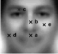
The face recognition schemes considered so far (PCA, Backpropagation) both use a low-dimensional, global, and non-topographic representation of faces to extract personal identity. A processing scheme which derives local topographic representations by introducing a general topographic kernel that projects signals to the subspace spanned by the PCA eigenmodes has been proposed by Penev and Atick. The procedure, termed local feature analysis (LFA), derives a dense set of local feed-forward receptive fields, defined at each point of the receptor grid, that is optimally matched to the input and whose outputs are as decorrelated as possible. The representation no longer satisfies the desirable condition of output decorrelation, which holds for the PCA representation, but can be enforced to satisfy the condition of minimum correlation. However, the LFA representation has the same best reconstruction, generalisation, and object constancy properties as the global PCA one. Figure 11 shows the results of applying the algorithm to an ensemble of aligned faces. The local receptive fields, which develop, resemble feature detectors for the mouth, nose, eyebrows, and the cheeks. To produce a local sparse-distributed representation the residual correlation between the outputs are further processed by lateral inhibition in a sparsifying neural network.
3.4 Independent Component Analysis
The template-based approaches described above (PCA; LFA), consider only second-order statistics of the image set, and do not address higher-order statistical dependencies such as the relationships among three or more pixels. A generalisation of PCA, known as independent component analysis (ICA), has been applied to a set of face images by an unsupervised learning algorithm which maximises the mutual information between the input and the output, thereby producing a statistically independent representation.
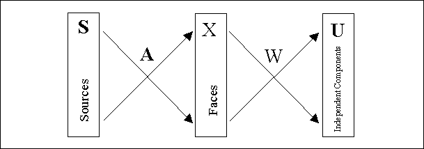
Figure 12 shows the general procedure for using ICA on a set of face images. The input images X are considered to be composed of linear combinations of unknown basis images S. The basis images are recovered using an unsupervised learning algorithm, which produces the statistically independent outputs U. Since the number of independent components found by the ICA algorithm corresponds to the dimensionality of the input, the original face images were transformed into a set of m linear combinations (m << N) of the N input images, thereby reducing the number of extracted independent components to m. For a recent review on independent component analysis techniques the reader is referred to Deco and Obradovic and Lee.
Most existing image analysis systems are based on the extraction of appropriate features or small-sized representations of the images, thus reducing the redundancy, as well as the dimension of the data to be further classified and interpreted by the system. Generation of a „good“ feature or small-sized image representation data set is a crucial aspect of the analysis or recognition procedure, requiring that as much as possible from the useful information of the original images be included in the derived feature data set. This requirement can ensure that small distortions in the shape of the objects shown in the images would not affect the subsequent feature-based classification process.
Multilayer perceptrons have been widely examined in the neural network field as a tool for image classification, based on appropriate feature extraction from the images. Apart from deterministic features, many statistical features, such as moments and linear prediction coefficients, have been used, e.g., for classification of textured images . A crucial aspect concerning the performance of multilayer network classifiers is generalisation, i.e. the ability of the network to classify correctly input data which were not included in its training set. Results from various applications have shown that good generalisation is a result of appropriate network design; a rather small network size can make the network learn incomplete solutions, while an unnecessarily large size may lead the network learn only the specific training samples and noise. A small number of interconnection weights (i.e. free parameters during training) should be generally used and any a-priori knowledge about the problem should be included in the network structure. Many good results have been obtained when structured networks are applied directly to image pixels. A multilayer network can, for example, accept an image representation directly in its input layer and be trained by some supervised learning algorithm, e.g., learning vector quantization or a backpropagation variant, to classify these representations in different categories.
However, real images always are of large size. Consequently, the required number of the classifying network interconnection weights, especially between the units of the first hidden layer and the network inputs, can be very large, resulting in prohibiting learning times, as well as in poor network generalisation. Since the optimal size of feedforward neural networks is generally an unknown quantity in most neural network applications, various techniques have been proposed for approximating it; pruning algorithms, including weight decay, weight elimination, weight sharing and receptive fields architectures, as well as constructive algorithms, including node or network splitting, and cascade-correlation types, are such examples. Nevertheless, simple use of such methods cannot provide an effective solution to the problem, mainly due to the large size of the input network layer, which generally equals the size of the image representation. It is, therefore, essential to combine the above algorithms with a reduction of the input layer size.
Multiresolution analysis is a possible tool for reducing the size of the image. Hierarchical neural networks can then be derived and used, so as to achieve a major reduction in the number of interconnection weights, as well as in the required learning times.
Representation of signals at many resolution levels has gained much popularity especially with the introduction of the discrete wavelet transform, implemented in a straightforward manner by filter banks using quadrature mirror filters (QMFs). In image processing the above are equivalent to subband processing. Image decomposition is performed with an appropriate filter bank, called (decimating) QMF filters. An appropriate bank of reconstruction (interpolating) QMF filters guarantees perfect reconstruction of the original image from its subband components. Multiresolution decompositions result in approximation images of low resolution that contain coarser information of the image content and in a set of detail images which contain more information as resolution is gradually increasing. Such decompositions are obtained as follows:
Using appropriate finite impulse response perfect reconstruction filters, which generally include a low-pass and a high-pass filter, we split the original image (level 0) into four lower resolution images, one of which is the approximation image at the lower resolution level (-1), and the three remaining ones are the detail images at that level. If this decomposition procedure is successively applied to the approximation images, we get a multiresolution approximation of the original image, providing images of continuously decreasing resolution and size .
Perfect reconstruction of the image at a particular level is achieved through synthesis of all four subband components, i.e., the approximation and the three detail images at the directly lower level. Perfect reconstruction filter banks have been developed based on the assumption that all subband signals are available and used in the reconstruction procedure. This is not, however, true, when only one of the subband image components is used for reconstruction; in this case perfect reconstruction filters lose their optimality. Nevertheless, feedforward neural networks can be used to compute optimal, analysis and synthesis filters through minimisation of the mean squared difference between the original and reconstructed images. Such networks contain one hidden layer, linear hidden and output units and operate in autoassociative form. During training, they are provided with the same input and desired images or image blocks; the low resolution image with the most important frequency content is constructed at the network hidden layer .
4.2 Hierarchical Multiresolution Neural Classifiers
Hierarchical neural network architectures constitute an efficient scheme for classifying multiresolution representations. A feedforward multilayer network can be trained first to classify an approximation image at a quite low resolution. An hierarchical network classifier is then sequentially constructed to handle the image at higher resolution levels. More specifically, after training a network, at say, resolution level j, to classify approximation images at that resolution level, the network performance is tested, using a validation set with approximation images at the same resolution level j. If the performance is not considered acceptable, training is performed at the next, i.e., the (j+1), resolution level; this procedure can be then continued, until reaching a resolution level where the network performance is satisfactory.
In this approach, it would be desired that the network at level (j+1) a-priori includes as much as possible from the „knowledge“ of the problem acquired by the former network at level j. Some early results in this topic suggested using the computed weights of the low-resolution network as initial conditions for the weights of the high resolution one. Another approach takes advantage of the fact that the information of the approximation image at level (j+1) is equivalent to the information included in both the approximation and detail images at level j. As a consequence, we can train three more networks, separately from the former one, to classify the detail images at level j and let the network at level j+1 contain in its first hidden layer a number of units equal to the union of the first hidden layer units of all four lower resolution networks. Formulae have been derived that permit transfer of the generally large number of (already computed) weights between the input and the first hidden layer of the low resolution networks in corresponding positions of the high resolution network. These formulae permit computation of the generally large number of weights between network’s input and first hidden layer be efficiently performed at lower resolution and be then fixed during training of the high resolution network. A small number of nodes is added to the first hidden layer of the network at level (j+1), and computation of the resulting new interconnection weights, as well as of the generally less complex upper hidden layers is performed by training the corresponding parts of the high resolution network. The above-mentioned addition of hidden nodes is performed sequentially during training, similarly to the cascade correlation methodology.
It should be mentioned that training and use of all four networks at level j is not always meaningful; this is due to the fact that in many cases only one of the four subband images contains the significant portion of the content of the original image. In such cases only the corresponding low resolution image should be used; the decomposition using optimally designed filters can help in creating and selecting the low resolution image with the highest information content. The performance of multiresolution hierarchical neural classifiers was examined in a pattern recognition application, where 2-D gray-scale images, with dimensions 34 x 49 pixels, had to be classified in two categories. Training a fully connected network at this resolution level, using weight decay, provided generalisation of only 86%. We used multiresolution analysis to reduce the input image size. The low resolution representations at level (-1) contained (21 x 29) pixels. We continued the decimation procedure one step more, obtaining low resolution representations of (15 x 19) pixels at level (-2). We then examined the performance of hierarchical network classifiers. We started by training a two hidden layer network at level (-2), using 8 and 4 hidden units respectively; the generalisation ability of it was found to be (80 %). By transferring the weights between the input and first hidden layer of this network to corresponding weights of the network at level (-1), subsequent training of the resulting network, and further increase of resolution to level 0, we constructed a network, whose generalisation capability was greater (92%) than the fully connected network at.level 0.
5. Features in Speech Perception
We highlight two broader domains surrounding specific attributions of emotion and the specific features of speech that underlie them, and argue for caution over compartmentalising these broader domains. It seems to be a general rule that variations in what we call the augmented prosodic domain (APD) are emotive - perhaps because they signal departure from a reference point corresponding to a well-controlled, neutral state. Our studies show that various departures from that reference point are reflected in the APD, including central and sensory impairments (schizophrenia and deafness) as well as emotion. Intuitively it seems right to acknowledge that departures from well-controlled neutrality are highly confusable, and it is unclear that phonetics should to try drawing those distinctions more sharply than listeners tend to. A system called ASSESS automatically measures properties in the APD, opening the way to explore it in an empirical spirit.
5.1. Emotion: In what Context?
Any interesting topic is worth approaching from more than one angle. We have come to the study of emotion from an angle that is somewhat different from that of most people. The result is a distinctive perspective, which we try to convey here. We regard it as a natural counterbalance to other approaches, expressing ideas, which ought to be kept in mind as a null hypothesis even if one chooses to follow an alternative approach.
The distinctive idea in our approach is that emotion is not a special problem: it is properly handled in the context of wider concerns. That idea applies at two levels. At the level of understanding listener responses, we have treated emotion as part of a wider domain concerned with evaluative judgements about speakers and reactions to them. At the level of understanding relevant speech variables, the variables that we have related to emotion form part of a domain that we will call the Augmented Prosodic Domain. We explain below what that entails.
We stress that we are not interested in doctrinal confrontations. We believe that our approach captures enough of the truth to be useful in a range of contexts. The same is almost certainly true of approaches, which focus more selectively on emotion. We assume that in the longer term more of the truth will be captured when approaches are formulated that combines the merits of both. In the meantime both approaches have practical uses.
Practically, our approach rests on a system called ASSESS. The core of ASSESS is a highly simplified representation of the speech signal based on a few features that we call landmarks. The main landmarks are peaks and troughs in the profiles of pitch and speech intensity and the boundaries of pauses and fricative bursts. These and a few other parameters define a representation of the speech signal which is equivalent to (and can be used to generate) a sketch of its main prosodic features.
The early stages of ASSESS generate this core representation automatically. There is nothing very profound about the methods that they use. They are chosen for robustness rather than quantitative precision. The later stages of ASSESS derive summary statistics from the core representation. Most of them are straightforward, dealing with attributes like the range and midpoint of rises and falls in intensity or pitch. A few are more sophisticated, like the parameters of the quadratic functions that best fit ‘tunes’ in the sample (a tune being the portion of the pitch contour that lies between two pause boundaries). The statistics also provide information on average spectra and spectral change, using the landmarks to find (e.g.) subspectra associated with intensity peaks (which tend to correspond to vowel centres).
The point of the approach is to capture a subset of the speech signal, which is intuitively natural and empirically significant. Intuitively, it summarises the output of channels concerned with prosody and some aspects of voice quality. For convenience, we will say that it deals with an augmented prosodic domain or APD for short. Its empirical significance is that information about that domain seems to account for a considerable proportion of the judgements and evaluations that people make on the basis of speech.
The problem that led us into the augmented prosodic domain was describing what happens to people’s speech when they lose their hearing. When we began work in that area, the literature tended to suggest that deafened people’s speech was not a problem. It did not generally become unintelligible, and nothing further needed to be said or done. Goehl and Kaufman underlined that view in a memorable exchange [, ].
Our experience with deafened people led to a different view: even when intelligibility is not a problem - and sometimes it is - there certainly is a problem with the reactions and impressions that deafened people’s speech evokes. Many of the reactions involve attributions of emotion.
We probed these reactions in a questionnaire study []. Factor analysis identified seven main themes in the response patterns. Of these three related to inferred emotions - warmth, social poise (which included lack of anxiety or timidity), and stability. The others were competence, plus motor disability, intellectual disability, and aversiveness. Judgements on all of these variables related to level of hearing loss. This is to say that speech variables, which actually reflected the limitations of control imposed by impaired hearing, were misinterpreted by listeners as signals of the speakers’ emotional makeup.
A predecessor of ASSESS suggested what the speech variables in question might be. Judged stability correlated with relatively slow change in the lower spectrum. Judged poise correlated with narrow variation in F0 accompanied by wide variation in intensity. Judged warmth correlated with a predominance of relatively simple tunes, a tendency for change to occur in the mid-spectrum rather than at the extremes and a low level of consonant errors (the last was established by phoneticians, not by the ASSESS-like analysis. Competence was associated with the pattern of changes in the intensity contour.
These measurements were made in the context of understanding deafness and its effects, and published accounts describe them in that context. However, they can also be set in the context of emotion. In that context, they make the point that the enhanced prosodic domain carries information about a range of speaker attributes. They also make the point that listeners do not fully disentangle the various factors that actually impinge on the domain - in particular, they do not disentangle the effects of impaired control due to hearing loss and emotionality.
ASSESS developed the idea that the kinds of measures which those studies had considered form part of a natural domain with recurring links to issues of emotion and evaluation. A large study which is currently under way applies ASSESS to deafened speakers in order to evaluate the effects of cochlear implants [, ]. The analysis confirms that the augmented prosodic domain is highly sensitive to differences between deafened speakers and controls. However, we have also applied the approach to other domains. One of the firsts was emotion per se.
5.3. ASSESS Applied to Emotion
Our study of emotion used passages constructed to suggest four emotions - fear, anger, sadness, and happiness. A fifth, emotionally neutral passage was used as a baseline. The passages were of comparable lengths, taking about 25-30 seconds each to read. Speakers were 40 volunteers from the Belfast area, 20 male and 20 female, aged between 18 and 69.
Recordings were digitised at 20kHz, after low pass filtering at 10kHz. ASSESS can estimate absolute intensity by using a calibration signal with a known dB level, but here no absolute referent was available, and level was normalised by treating the opening of a passage as a referent and setting its median intensity at 60dB. This seems unlikely to confound results. Technical information on statistics is given elsewhere [].
There was wide range of differences between passages - over 1/3 of the measures considered yielded significant differences. The challenge is to reduce these to a manageable set. The largest set of differences reflect an effect that distinguishes two broad groups of passages: afraid, angry and happy on one hand, sad and neutral on the other. They involve intensity contrasts. It seems apt to call the groups intensity marked and intensity unmarked respectively. Table 1 shows the main features of the effect. Measures are in bold face if they are significantly different from the neutral passage. The first two columns show intensity measures for all points outside pauses. These global measures are higher for fear, anger and happiness than for sad and neutral passages. However, intensity marking is not a simple matter of loudness. ASSESS reveals two types of structure in it.
mean median peaks troughs
Anger 64.11 61.57 66.87 59.97
Fear 63.64 61.51 66.45 59.57
Happiness 63.38 61.59 66.07 59.52
Sadness 62.42 60.32 65.10 59.12
Neutral 62.33 60.73 64.87 58.83
p 0.000 0.003 0.000 0.095
Table 1: Selected intensity contrasts between groups.
First, note that intensity is normalised. Hence the first two columns do not mean that the first three emotions are associated with louder speech: it means that intensity rises after the first few phrases. This may be called a crescendo effect.
Second, note that the effect is more marked with means than with medians. That suggests it involve stretching in the top end of the intensity distribution rather than just a global upward shift. The inference is confirmed by the last two columns. The contrast in the level of peaks in the intensity contour is even more marked than the contrast in overall mean. However, there is much less contrast in the level of troughs (that is, minima).
Pauses were longer in the intensity marked passages, most markedly so in happiness and sadness. This is consistent with the general pattern of heightened dynamic contrast in the intensity marked passages. Several other features distinguish intensity marked passages from the neutral passage, and to a greater or lesser extent distinguish them from each other.
Rises Falls Tunes Plateau
Median median median IQR
Fear 82.35 84.8 1265 10.8
Anger 81.66 80.5 1252 10.2
Happiness 78.03 77.4 1404 8.2
Neutral 78.50 77.2 1452 8.4
Sadness 77.28 81.4 1179 11.0
P 0.000 0.000 0.001 0.006
Table 2: Duration features and negative emotions (ms).
Properties involving the duration of intensity features may tend to signal negative emotions: they do not affect happiness, and they may affect sadness. Table 2 summarises the data. The duration of amplitude movements distinguishes fear and anger from the neutral passage again. Both have longer median duration for both falls and rises. But in contrast to the crescendo and intensity stretching effects, this effect is stronger in fear than anger. Protracted intensity falls also characterise sadness. The duration of tunes show a similar pattern. Also broadly similar is a property of intensity plateaux. The interquartile range of their duration increases markedly in fear and sadness, and less so in anger.
The passages differ in the distribution of energy across the spectrum, but few of the effects are easy to interpret.Most straightforwardly, all the emotions are characterised by greater variability in the duration of fricative bursts (as measured by the standard deviation) than the neutral passage.
A second clear effect involves anger. Here the average spectrum for non-fricative portions of speech has a high midpoint. That is not surprising: it parallels a well-known effect of tension on spectral balance []. Conversely, the sad passage gives a significantly lower spectral midpoint than any of the intensity marked passages - it is lower even than the neutral passage.
Fricative bursts are associated with a number of effects, which seem paradoxical at first sight. Anger is associated with high average energy in fricative bursts, but the average spectrum for slices classed as fricative has a low mean and a markedly negative slope. The implication appears to be that the intensity associated with frication is not rising as fast as the intensity associated with the lower spectrum. Fear and happiness are distinctive in terms of the subspectrum which shows variability in slices classed as fricative. These too show markedly negative slopes, indicating relatively low variability in the regions associated with frication. The effects may be less to do with frication than with raised variability in the lower spectrum.
Two aspects of the pitch contour show differences - the distribution of pitch height and the timing of pitch movement. Passages do not differ significantly in pitch height per se. However, they do differ in its distribution. Again, the differences, which are clearly significant, fall into an orderly pattern. All of them involve interquartile intervals, which can be thought of as measures of the range a measure usually occupies. When all pitch inflections are considered together, the passage difference in interquartile interval just reaches significance. Separating maxima and minima shows a weak passage effect for minima and a much stronger one for maxima. In all three cases, range is widest for happiness and nearly as wide for anger, with the lowest range in the neutral passage.
Afraid Angry Happy Sad
Spectrum
midpt & slope + –
Pitch movement
range + +
timing + +
Intensity
marking + + +
duration + + +
Pausing
total + +
variability +
Table 3: Summary of distinctions among passages
All the distinctive pitch duration features are associated with happiness. Pitch plateaux are shorter in the happy passages than elsewhere, and their durations generally lie within a narrower range (as measured by the inter quartile range). Conversely, pitch falls last longer in the happy passage than in the neutral one. This also happens in the sad passage. Pitch rises are also significantly faster in the happy passage than in the neutral passage. The overall picture is that happiness involves pitch movement, which is not only wide, but constant.
Table 3 provides a compact outline of the findings. This shows that features in the augmented prosodic domain distinguish each of the passages from any other in several ways.
5.4. Prosody in ‘Flattened Affect’
Our study of emotion is a module within a larger clinical project concerned with the attributes of speech that differentiate schizophrenics from normal speakers. Clinicians’ judgements about speech are a key element in diagnosis [,], particularly in the context of ‘flattened affect’, which is linked to poor prognosis and hospitalisation [,]. It is obviously a matter of concern that diagnosis might be influenced by individual differences in clinicians’ aptitude for impressionistic judgements about speech. We studied the possibility of providing objective measures for that reason.
Our schizophrenic sample consists of 72 subjects from Belfast who have a diagnosis of schizophrenia (DSM-III-R)[] of more than one year’s duration. At the time of testing 40 were outpatients who were attending a local psychiatric outpatient clinic and 32 were long-stay inpatients in a psychiatric hospital. The passages that they read were the same as the passages used in the study of emotion, and they were compared with the controls whose results have been outlined above.
Two broad types of comparison are worth drawing. The first involves contrasts between schizophrenic and control subjects in the delivery of an emotionally neutral passage. The second involves contrasts in the way that they differentiate between neutral passages and passages with strong emotional content. The approach that we have taken allows both to be made within a single framework, because it treats the expression of emotion as part of a broader descriptive task.
Comparing schizophrenics and controls on the neutral passage, several significant contrasts emerge. Schizophrenics showed higher mean F0, along with lower pitch variability in terms of both the amounts by which pitch tended to rise between neighbouring minima and maxima, and the amount by which tunes tended to differ in their central pitch. The way they varied intensity was more stereotyped: both rises and falls in intensity showed a narrower range of variation than in controls, as did the duration of falls in intensity. Conversely, they showed increased variability in the duration of silences.
The variables involved in these contrasts are emotion-like. As the term ‘flattened affect’ suggests, they convey something like absence of any emotional colour, even the tints that we expect in so-called neutral speech. But it is not clear how accurate that is. The second comparison underlines uncertainty whether the issue is the existence of emotion or its expression.
Table 4 is parallel to Table 3, but it juxtaposes the contrasts between neutral and emotional passages in controls (C columns) and patients (P columns). Most of the entries are self-explanatory. The pattern of intensity marking is worth commenting on - the crescendo effect is absent in the cases where controls show it, but the opposite effect - a diminuendo - occurs in sadness, where the controls show level pitch.
Afraid Angry Happy Sad
C P C P C P C P
Spectrum
midpt & slope + + – :
Pitch movement
range + : + +
timing + : + :
Intensity
marking + : + : + : : -
duration + + + + + +
Pausing
total + : + +
variability : + : + : + + +
Table 4: Patient and control distinctions among passages. Colons mark effects that are absent in one group but not both.
The nature of schizophrenia is controversial, but whatever the underlying disorder is, it generates disturbance in the APD. That conveys something about the speaker’s state to listeners. Conversely when these patients try to express emotion, there are changes in the APD domain, but the balance of markers is not a normal one.
We have drawn attention to two broader domains surrounding specific attributions of emotion and the specific features of speech that underlie them, and highlighted reasons for caution about compartmentalising these broader domains.
It seems to be a general rule that variations in the augmented prosodic domain are emotive. That may be because they signal departure from a reference point corresponding to a well-controlled, neutral state. Various departures from that reference point are reflected in the augmented prosodic domain, including central and sensory impairments as well as emotion. We have some evidence that stylistic and dialect variations, which intuitively also seem to be emotive, are also reflected in the augmented prosodic domain [4,]. Intuitively it seems right to acknowledge that departures from well-controlled neutrality are multidimensional and highly confusable. It is often genuinely difficult to know whether somebody is angry or depressed or preoccupied or simply hoarse. On one hand, it is asking too much to expect phonetics to draw those distinctions when listeners cannot: on the other, it is failing to represent the fluidity of the categories in which representations of the speaker are couched. A cynic might add that the notorious difficulty of finding pure and natural samples of emotional speech reinforces the case.
That kind of view suggests a programme of inquiry, which is thoroughly empirical, concerned with documenting the broad patterns of variation that occur in the augmented prosodic domain and the ways in which they are received. ASSESS reflects the fact that contemporary technology makes that kind of programme practical.
Figure 13 presents traces from an individual speaker (C14) - arbitrarily chosen from the group studied by McGilloway - and shows how they relate to the kind of feature set suggested by ASSESS analysis. Panel (a) - (e) summarise the output of initial processing on each of five passages - one neutral, and four expressing specified emotions (anger, fear, happiness and sadness). The heavy lines in each panel show signal amplitude (referred to the left-hand scale, in dB), the light lines represent pitch (referred to the left hand scale, in Hz). Timescale (on the horizontal axis, in milliseconds) is adjusted to let the whole passage appear on a single screen. The patterns are summaries in that inflections and silences have already been identified from the raw input, and the overall contours are represented by a series of straight lines (or gaps) between the resulting points. The ASSESS summary at this stage also generates several spectrum-like representations, but they contribute relatively little, and they are not shown.
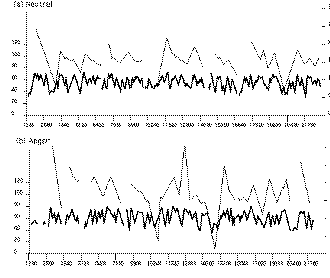
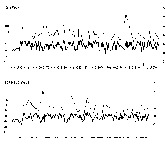
Figure 13 Output of initial processing on each of five speech passages
It is not self-evident from inspection that the contours differ systematically, but extracting features of the kind considered by ASSESS indicates that they do. Figure 14 shows how C14's speech relates to the general distinctions found in the whole subject group (n=40). Each caption on the left hand side refers to an ASSESS output feature whose value in one or more emotional passages is significantly different from its value in the neutral passage. The features are selected from a much larger number that McGilloway has shown meet that basic criterion. Selection is geared to (a) avoiding redundancy, (b) representing the main logically distinct areas where differences occur, and (c) achieving some formal consistency (e.g. using centile measures to describe central tendency and spread).
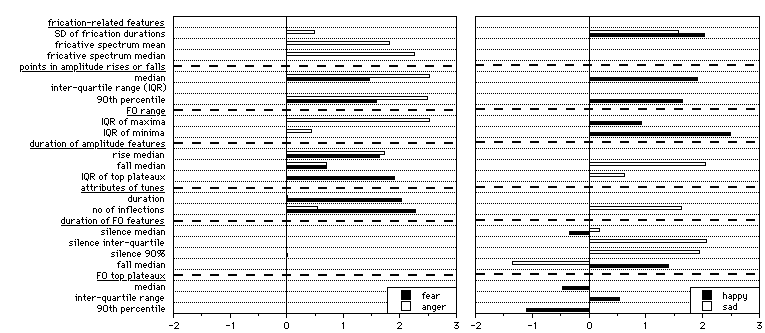
Figure 14 Relation of C14's speech to the general distinctions found in the whole subject group (n=40). See text for furter details.
The graph shows the fit of C14's data to a template based on the overall analysis. A bar is present if the feature in question differentiates the emotion in question from the neutral passage in the overall analysis. Its direction is positive if the difference is in the direction indicated by the overall analysis. Its length is proportional to the difference between the feature value for the emotion in question and the feature value for the neutral passage, relative to the standard deviation of the values for all five expression categories (four emotions plus neutral) on that feature.
The main points to be made from panel f are that ASSESS-type automatic analysis generates a range of features that are relevant to discriminating emotion from neutral speech, and that different emotions appear to show different profiles. It remains to be seen how reliably individual passages can be assigned to particular emotion categories, but there are grounds for modest optimism. A more detailed description of the ASSESS system can be found in the appendix.
This report presented results of extracting linear and non-linear features from visual and auditory signals. In particular we presented results on:
A supposition for satisfying recognition results is the good alignment of the faces to a general viewpoint. Therefore we reviewed general schemes for face detection and normalisation in chapter 2, which could be used to normalise the images from an un-normalised dataset, or from real-time video data. We have presented several template-based approaches for face and expression recognition on static images, some of which were used to study their performance on a public available face dataset in chapter 3.2. To normalise the face images used in the study, we employed our own normalisation algorithm, which has to be expanded to cope with more general viewing positions of faces in real-world scenes. In chapter 4 an outlook of the use of multiresolution hierarchical neural networks for vision is given.
Since the analysis of emotional speech can already be performed by the ASSESS system, we presented the application of the system in a psychological study in chapter 5, followed by a brief description of the system in chapter 6. A more technically description of the ASSESS system can be found in the appendix.
Next, after completion of the feature extraction task from image sequences, both systems need to be combined, resulting in a fully working audio-visual emotion recognition system. To complete the feature extraction task, the normalisation procedure has to be expanded and made real-time capable. Further, a good database is needed including multiple sequences of facial expression with synchronised speech to develop and test the feature extraction software.