Medial Features
We present a local feature detector that is able to detect regions of arbitrary scale and shape, without scale space construction. We compute a weighted distance map on image gradient, using our exact linear-time algorithm, a variant of group marching for Euclidean space. We find the weighted medial axis by extending residues, typically used in Voronoi skeletons. We decompose the medial axis into a graph representing image structure in terms of peaks and saddle points. A duality property enables reconstruction of regions using the same marching method. We greedily group regions taking both contrast and shape into account. On the way, we select regions according to our shape fragmentation factor, favoring those well enclosed by boundaries - even incomplete.
We achieve state of the art performance in matching and retrieval experiments with reduced memory and computational requirements. Please visit Medial Feature Detector for executable code and documentation.
 |
 |
 |
 |
| (a) | (b) | (c) | (d) |
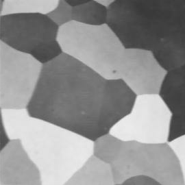
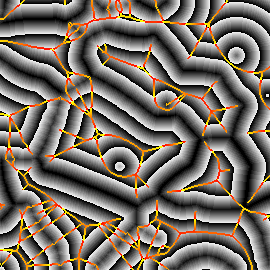
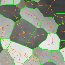
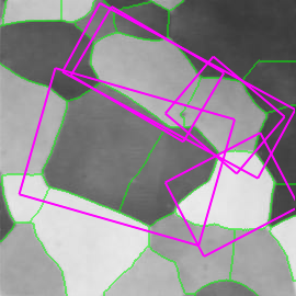
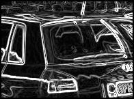
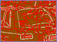
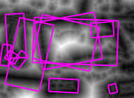
Figure 1. Medial feature detection. (a) Input image. (b) Weighted distance map and medial axis. The color map indicates ascending direction by (black $\rightarrow$ white) and (yellow $\rightarrow$ red) transitions, respectively. (c) Image partition. (d) Regions detected.
Fig. 1 gives a preview of our result. No edges are needed; the distance map is computed directly on image gradient. It is weighted by the gray level of the gradient, but propagation obeys the Euclidean distance, evident e.g. at the top-right of Fig. 1(b). A weighted medial axis is computed on the entire image representing its structure as a graph. With a dual operation, labels are backpropagated to give a partition as shown in green lines, guided by a decomposition of the medial axis at saddle points of the distance map. The latter are exactly the points where the medial axis meets partition boundaries in Fig. 1(c).
Graph vertices are constructed at distance peaks in region interior, and edges at saddle points on region boundaries. The partition is sensitive both to contrast, represented by gradient strength, and to shape; regions are separated even where intensity is uniform. Both elements are captured in edge weights, guiding a region grouping process whereby candidate features are generated. The features, as shown in Fig. 1(d), are selected according to our shape fragmentation factor. The latter measures how well a region is enclosed by boundaries, in agreement with the Gestalt principle of closure. Incomplete boundaries are allowed, as well as independent selection of whole regions and their parts.
Given an image $f$ defined in domain $X$, we define the weighted distance map $h = D(f)$ of $f$ as $h(x) = \bigwedge_{y \in X} \|x - y\| + f(y)$ for $x \in X$, where $\wedge$ denotes infimum and $\|\cdot\|$ the Euclidean norm. This definition is equivalent to infimal convolution or weighted erosion. Although it applies to arbitrary functions $f$, if the problem at hand is region detection in images, we use a function that is related to boundaries. In particular, given an input image $f_0$, a simple approach is to compute the gradient magnitude $g = |\nabla f_0|$ and then define $f(x) = \sigma / g(x)$ for $x \in X$, where $\sigma$ is a scale parameter. This generalizes the $0/\infty$ indicator function used in binary distance transform.
We compute the weighted distance map using our exact group marching (EGM) algorithm, a variant of group marching (GMM). The latter is a linear-time fast marching method that selects a number of points on the propagating front to move as a group, thus avoiding the cost of sorting. We move all points of the front as a group using a constant-time priority queue on quantized distance. Points at the same priority level are processed in arbitrary order, so this part of the computation can be made parallel. However, due to the Euclidean assumption and a bidirectional update, the entire computation is exact. It is also linear in the number of pixels.
 |
 |
 |
 |
| (a) | (b) | (c) | (d) |
Figure 2. (a) Input image, detail of leuven scene. (b) Gradient map. (c) White: source; red: medial axis; black: saddle point; blue: image boundary. (d) Weighted distance map, with detected features in overlay.
For each point $x \in X$, EGM also computes the source set $S(x)$. Informally, $S(x)$ is the set of points $y \in X$ for which the quantity $\|x - y\| + f(y)$ is minimized; a more precise definition is given in our ICCV paper. This set is used in the definition of medial axis below. Further, the source set $S(f)$ of the entire image $f$ is defined as the set of all source points of $f$. Source points are in general located at or near boundaries. We show that the distance map $D(f)$ is uniquely determined by the restriction of $f$ on its source set. Fig. 2 shows an example of weighted distance map along with source points, medial axis and detected features. The image gradient is used as an input.
Given the previous definitions of sources in a weighted distance map, we say that $x \in X$ is a medial point of $f$ if it has at least two distinct sources. The (weighted) medial axis $A(f)$ is the set of all such points: $A(f) = \{ x \in X : |S(x)| > 1 \}$. The source set and the medial axis of an image are mutually exclusive.
Our weighted medial axis (WMA) algorithm computes the medial axis $A(f)$ of image $f$ given its weighted distance map $D(f)$ and source set $S(f)$. We show that the medial axis function is associated to peaks (local maxima) and ridges of the distance map. Hence we begin computation at such points and continue propagating along $A(f)$ based on spatial connectivity and a residue function $r(x)$.
The residue function is a means to deal with singularities of the discrete domain and is a generalization of the chord residue by Ogniewicz and Kubler. The latter is defined for binary shapes, as the difference between the length of a boundary curve segment and the corresponding chord length in a circle that is contained in the shape and bitangent to the boundary curve at the two endpoints. We see the distance value as a third dimension, or height. We thus generalize circles to cones lying below and bitangent to a particular set of curves in three dimensions.
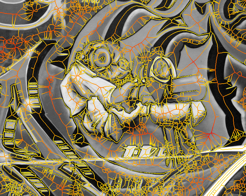
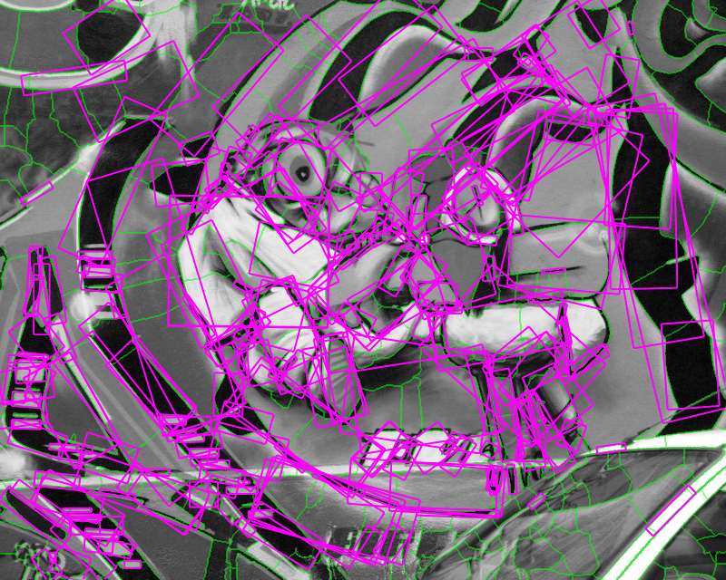
Figure 3. Left: medial axis for graffiti scene image 1. Minimum (maximum) height on the medial axis is mapped to yellow (red), as in Fig. 1. Right: detected features and underlying partition.
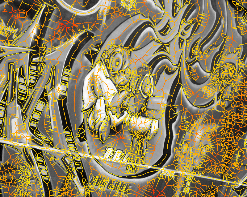
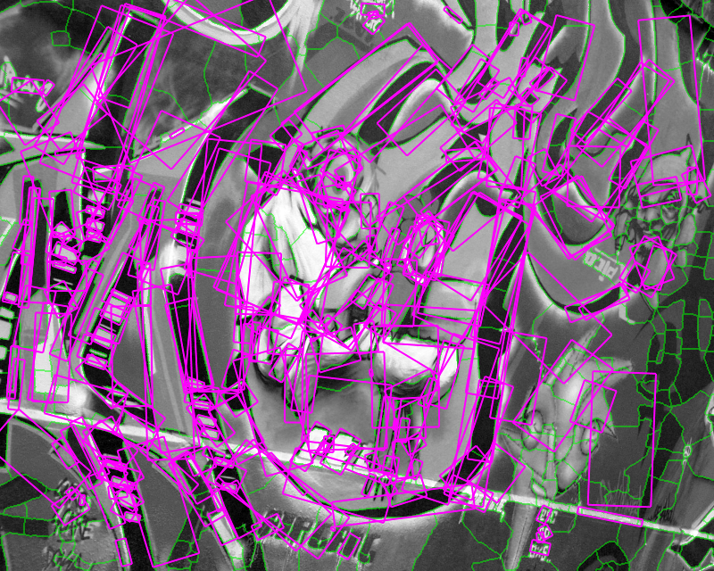
Figure 4. The same experiment with Fig. 3, but for image 3 of the graffiti scene. The medial axis appears to have changed form, but the features are quite stable.
Using a graph to represent the topology of the source set, we make it possible to compute the residue function $r(x)$ in constant time. Hence we show that WMA is linear in the number of pixels on the medial axis, which in turn is only a small fraction of the number of pixels in the image. We also guarantee that the resulting medial axis is connected. Figures 3,4 show examples of what our weighted medial axis looks like on a gray-level image. They also show the detected features, as defined below.
While the medial axis typically represents the shape of single object, we represent the structure of an entire image. We decompose it into components and construct a weighted graph $G(f)$ with the following properties: (a) vertices correspond to local maxima (peaks) of the distance map; (b) edges correspond to local minima along the medial axis (\ie, along ridges), therefore to saddle points of the distance map; (c) the weight of each edge is defined as the height at the associated saddle point.
Our medial axis decomposition (MAD) algorithm constructs graph $G(f)$ given the distance map $D(f)$ and the associated medial axis $A(f)$. We start with the distance peaks on the medial axis, and continue propagating downwards. We assign a component label $\kappa(x)$ to each $x \in X$, represented by a graph vertex. We build $G(f)$ by gradually inserting a vertex whenever we first visit a peak with unlabeled neighbors, and an edge whenever two fronts with distinct labels meet. Propagation is equivalent to the watershed segmentation of the negated distance map restricted to the medial axis, with peaks as markers. It is topological but based on a distance function that is also contrast-weighted.
Next, we partition the entire image via a reconstruction operation. We exploit a duality property whereby this operation reduces to EGM algorithm. In particular, given distance map $h = D(f)$ and medial axis $A(f)$, we invoke EGM with input function $g(x) = -h(x)$ if $x \in A(f)$, or $+\infty$ otherwise. Effectively, we backpropagate from the medial axis to the boundaries. Further, we use labels $\kappa$ from MAD and construct component labels $\kappa(s(x))$ for $x \in X$, where $s(x)$ is any representative of the source set $S(x)$ under the new backpropagated distance. This label map provides a partition of domain $X$. As illustrated by green boundaries in Fig. 1,3,4, this partition is equivalent to watershed segmentation of the negated distance map $-h$ on $X$ with the components of MAD as markers. However, casting it as distance propagation enables the use of EGM, hence a very fast implementation.

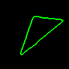
Figure 5. Left: binary input image (no gradient used here). Middle: point labels; color legend is the same as in Fig. 2. Right: image partition. There are two saddle points on the medial axis, and two gaps of width $w_1$, $w_2$. The fragmentation factor of triangle $\kappa$ is $\phi(\kappa) = (w_1^2 + w_2^2) / a(\kappa)$ where $a(\kappa)$ is its area.
We define a feature to be the union of any number of adjacent components. We group components in non-increasing order of edge weights, using the union-find algorithm. Each newly acquired component is considered as a potential feature, according to a shape criterion. For each edge $e$ of graph $G(f)$, let $x(e)$ be the saddle point where $e$ is generated. This point corresponds to a boundary gap of width $w(x(e))$, which is easily computed in constant time. Given component $\kappa$ with area $a(\kappa)$ and incident edge set $E(\kappa)$, we define its shape fragmentation factor as $ \phi(\kappa) = \frac{1}{a(\kappa)} \sum_{e \in E(\kappa)} w^2(x(e))$. As shown in Fig. 5, this factor measures how well a region is enclosed by boundaries, which may be incomplete. Hence it captures the Gestalt principle of closure. Finally, we select a component $\kappa$ as an image feature if $\phi(\kappa) < \tau$ where threshold $\tau > 0$ controls the selectivity of the detector.
The first experiment involves matching across viewpoint, zoom, rotation, light, and blur. We measure performance in terms of repeatability and matching score. Fig. 6 presents measurements of our medial feature detector (MFD) compared to Hessian-Affine, Harris-affine, MSER, IBR, EBR and Salient Regions, using SIFT descriptors for all detectors. MFD achieves excellent matching score, while repeatability is also high in most cases. Good performance is accompanied by a reasonably small number of responses, still providing good image coverage. Thanks to shape fragmentation, highly textured areas do not give any response.


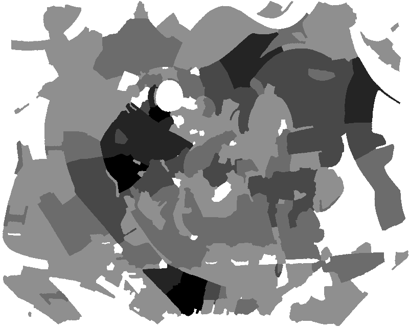


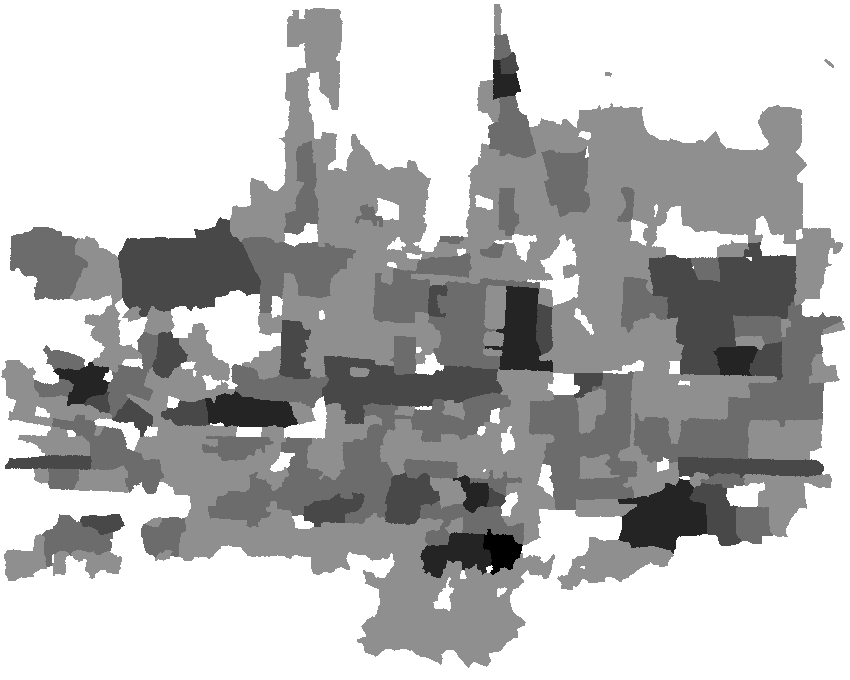


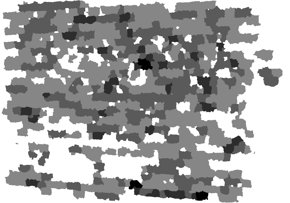
Figure 6. Left column: repeatability, middle column: matching score, right column: coverage for image 1. From top to bottom, (scene / #features in image 1 / detection time): (graffiti / 530 / 0.55 sec), (boat / 665 / 0.72 sec), (wall / 876 / 1.08 sec).
The second experiment involves larger scale retrieval using a bag of words (BoW) model and fast spatial matching (FastSM), measuring performance in terms of mean Average Precision (mAP) score. Here we use the Oxford 5K dataset, comprising 5,062 images with 55 queries. We extract features and construct 50K and 200K vocabularies. We construct an inverted index and rank images with TF-IDF. Tables 1,2,3 present statistics on indexing space, average query time, and mean average precision, respectively. Indexing space and query time depend on the average number of features per image, and the objective is highest mAP with reasonable space/time requirements. MFD outperforms all detectors in terms of retrieval performance, followed very closely by Hessian-affine. The latter is however quite impractical in terms of memory and query times.
 |
 |
Table 1. Total number of features in Oxford 5K dataset, and features used in vocabulary construction. Total memory required for the inverted index, for the 50K and 200K vocabularies. |
Table 2. Average query time in msec. Inverted index refers to total TF-IDF ranking time; re-ranking to FastSM per image pair. |

Table 3. Mean average precision, with and without re-ranking.
Please visit Medial Feature Detector for executable code and documentation.
Publications
Conferences
[ Abstract ] [ Bibtex ] [ PDF ]